Technical report: Naive methods for estimating the causal effect in multiple treatment setting
Introduction
Causal inference allows us to estimate the causal interactions between random variables. It enables us to ask questions such as: “Does some medication lowers blood pressure?”. Throughout this post I will describe a project with the goal of estimating the causal effect in a multiple treatment setting (e.g., given a number of medications, which one lowers blood pressure most significantly). While the common framework in causal inference considers a binary treatment setting, in this post we will consider a multiple treatment setting, where the number of treatments can be larger than two.
Background (Potential Outcomes)
Considering the binary treatment setting, Neyman-Rubin’s potential outcome framework [2] is defined as follows:
Let \( X_i \in \mathbb{R^m} \) denote the covariates vector (i.e., pre-treatment covariates, or features), \( T_i \in \{ 0, 1\} \) denotes the possible treatments (e.g., control and treated groups), and let \( Y_i \in \{0,1 \} \) denote the outcome, for each sample \( i= 1,…,N \) in our trial.
Following the blood pressure example, $X$ might obtain patient indicators (e.g., gender, age, etc.), $T$ indicates whether the patient took the suggested medicine or not, and $Y$ can represent an increase or decrease in blood pressure.
Moreover, let $Y_{i0}$ denote the unit’s outcome had they been subjected to treatment T=0, and let $Y_{i1}$ denote the unit’s outcome had they been subjected to treatment T=1. These fixed quantities ($Y_0, Y_1$) are known as potential outcomes. Usually, for each sample we can only observe one of the outcomes but not both. Therefore, as also noted in [2] - causal inference is a missing data problem, and its main challenge is to estimate the missing potential outcome.
To measure the treatment effect for an individual unit $i$ we subtract the outcomes as follows: $Y_{i1}-Y_{i0}$, while for estimating the Average Treatment Effect we utilize expectation over the outcomes difference:
Framework for Multiple Treatments
Consider now \( k \) treatments that a subject may receive, let \( \mathbb{T} = \{ t_1, …, t_k \} \) be the set of possible treatments. For each subject, we may observe \( k \) different potential outcomes: $\{Y_i(t_1), ….Y_i(t_k) \}$. To estimate the causal effect in multiple-treatment setting, the following assumptions are required to hold:
- Stable Unit Treatment Value assumption (SUTVA) for multiple treatments - i.e., for each subject, the set of potential outcomes is identical and there are no “hidden” treatments which may lead to a different unknown outcome.
- Consistency assumption for multiple treatments (see note below for binary setting) extends to: \( Y_{i} = I_{i1} * Y_i(t_1) + … + I_{ik} * Y_i(t_k) \), where $I_{ik}$ denotes an indicator function which gets 1 whether subject $i$ received treatment $k$ and 0 otherwise.
Additionally, we require the treatment assignment mechanism to be individualistic (i.e. the $N$ subjects represent a random sample from an infinite population), and to satisfy ignorability (no unmeasured confounders):
Or in words, the potential outcomes are independent of the treatment assignment, conditioned on observed covariates X.
Lastly, we demand the assignment mechanism to be probabilistic (the common support assumption):
For the binary setting, the treatments domain is defined as \( T_i \in \{ 0, 1\} \) and the consistency assumption indicates that \( Y_{i} = (1-T) * Y_{i0} + T * Y_{i1} \) for all \( i \in \{ 1,…, n \}\).
Generalized Propensity Score
The probability for a treatment assignment $T=t$ given $X=x$ is noted as $r(t, X)$, and is also referred to as the Propensity Score (or Generalized Propensity Score - GPS, in the case of multiple treatments). More formally:
Under these assumptions, we can compare subjects with similar GPS and expect well estimated effects. Usually, $R(X)$, the GPS vector, is unknown, however we may estimate it with any statistical method.
To enforce the common support assumption, one may use the estimate $\hat{R(x)}$ to trim subjects which do not rely in the rectangular common support boundaries [1]. Specifically, for each treatment group $t \in \mathbb{T}$ we measure lower and upper bounds values for the GPS:
where $r(t, X | T = j)$ is the treatment assignment probability for $t$ among those who received treatment $j$. Once we compute these bounds, we can discard from our dataset subjects which do not rely in the range , according to the treatment each subject received. The effect for enforcing this assumption can also be illustrated in Figure 1.
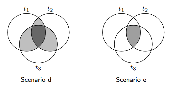 Figure 1: The common support assumption - we move from Scenario d to Scenario e by removing samples which
do not satisfy the common support assumption, illustration borrowed from [1].
Figure 1: The common support assumption - we move from Scenario d to Scenario e by removing samples which
do not satisfy the common support assumption, illustration borrowed from [1].
Finally, after dropping non eligible subjects, we shall re-estimate $\hat{R(x)}$ to get more accurate propensity scores. We may also repeat this for several cycles until we are satisfied, however, we should take into account the number of samples left for estimation while repeating this process.
Methods
To estimate the causal effect, we experiment with two types of methods, the first is known as Covariate Adjustment, and the second is Matching. We will describe shortly each of these methods while considering the binary setting for simplicity.
Covariate Adjustment
Under the ignorability assumption (and law of total expectation) it holds that: $E[Y_1-Y_0] = E_{x \sim p(x)} [E[Y_1|T=1, x] - E[Y_0|T=0, x]]$. Therefore, as follows from the consistency assumption, we may fit a model $ f(x, t) \approx E[Y|T=t, x] $ to estimate the ATE:
Notice that $f(x, t)$ explicitly models the relationship between treatment, covariates and outcome, thus, it might be more prone to errors. This method can be extended to use two learners, where each one of the learners models a single treatment group. We use the notation of S-Learner for a single learner, and T-Learner for two learners. In our experiments we examine both variants. Lastly, these methods are also reviewed in [5] who introduced X-Learner, a specialized learner for cases of unbalanced trials (i.e., where one treatment group is relatively larger than the other groups).
Following is a Python code sample for estimating the ATE with Covariate Adjustment (using a single learner):
def ate_by_covariate_adjustment(X: pandas.DataFrame,
                                y: pandas.Series,
                                treatment: int = 1) -> float:
    clf = SomeClassifier()
    clf.fit(X, y)
    treated_samples = X[X['treatment'] == treatment]
    control_adjusted_samples = deepcopy(treated_samples)
    control_adjusted_samples['treatment'] = 0
    control = clf.predict(control_adjusted_samples)
    treated = clf.predict(treated_samples)
    ate = numpy.mean(treated - control)
    return ate
Matching
This method estimates the causal effect by matching samples to their nearest neighbour, with respect to some distance metric. For each sample $i$ with outcome denoted as $y_i$, we define the estimate for the Individual Treatment Effect (ITE) as $\widehat{ITE}(i) = y_i - y_{j}$ when sample $i$ is in the treated group (i.e., $t_i=1$), or $\widehat{ITE}(i) = y_{j} - y_{i}$ when sample $i$ is in the control group (i.e., $t_i=0$), where sample $j$ belongs to the opposite group. Sample $j$ is the nearest neighbor of sample $i$, and its outcome is denoted by $y_{j}$. Examples for metrics that measure distance between two samples include Manhattan distance, Euclidean distance, etc.
Once we estimate the individual effect for each sample, we may also estimate the ATE:
When using Matching, it is common to limit the minimal distance value between two close samples. When following this mechanism, we denote the maximal distance value we allow as Calipher. Note that in this case some samples may have no match. In our trials we experiment with a few values of Calipher, and also without any limit (denoted as ‘None’ in the results section).
A basic implementation for computing the ATE estimate with matching (without Calipher):
def ate_by_macthing(X: pandas.DataFrame,
                    y: pandas.Series,
                    treatment: int = 1) -> float:
    control_mask = X['treatment'] == 0
    treated_mask = X['treatment'] == treatment
    control = X[control_mask]
    treated = X[treated_mask]
    control_target = y[control_mask]
    treated_target = y[treated_mask]
    distances: numpy.ndarray = some_distane_function(treated, control)
    matches = numpy.argmin(distances, axis=1)
    ate = numpy.mean(treated_target - control_target[matches])
    return ate
Extension to multiple treatments
For Covariate Adjustment, in the case of S-Learner we use one model for the complete treatments domain. While for T-Learner we actually fit a model for each treatment group.
In the case of Matching, each treatment group is compared to their most nearest samples from the control group.
# a snippet to naively estimate ATE in a multiple treatment setting
treatments: List[int]
for t in treatments:
    for estimator in [ate_by_covariate_adjustment, ate_by_matching]:
        print(t, estimator.__name__, estimator(X, y, t))
Dataset
For our experiments, we generated a synthetic classification dataset with 5 treatments, where one of them is kept as the control treatment (denoted with $t_0$), and the others are denoted with $t_i$ (where $i \in \{ 1,..,4 \}$) for each treatment group. In this technical report we choose to estimate the Average Treatment Effect (ATE) of $Y(t_0)$ vs. $Y(t_i)$, resulting in a total of 4 ATEs. The dataset is composed of the true ATE values which will allow us to evaluate our ATE estimates. Additionally, we experiment with two variants of the original dataset, one with all subjects, and another with only eligible subjects according to the rectangular common support. The true ATE values and number of subjects for each treatment group, in each of the datasets, can be observed in Table 1.
The full dataset has $46,700$ subjects, with $22$ covariates. After dropping non-eligible units we are left with $31,984$ units.
As noted earlier, the dataset represents samples from 1 control group and 4 treatments groups, while our targets domain is $\{ 0, 1\}$ for each sample.
The covariates are all numeric and comprised of 5 informative features (for classification), 5 irrelevant features, and 12
more features which are correlated with the treatments causal effect. We can choose positive, or negative effects for each treatment, in our trials the effects were all chosen as positive.
To generate the dataset we assisted with the CausalML [3] framework which provides a method for this goal: make_uplift_classification.
Lastly, since the common support assumption reduces our dataset to samples which have an equal chance for receiving all treatments, we had to intentionally sub-sample parts of the data to cause imbalances, for allowing this enforcement to have some effect on the performance.
| Treatment Group Key | True ATE (All) | # Subjects (All) | True ATE (Eligible) | # Subjects (Eligible) |
|---|---|---|---|---|
| control group (treatment 0) | 0.000000 | 9899 | 0.000000 | 4189 |
| (control vs.) treatment 1 | 0.012072 | 9775 | 0.011070 | 5691 |
| (control vs.) treatment 2 | 0.025728 | 9484 | 0.028199 | 6064 |
| (control vs.) treatment 3 | 0.053787 | 9017 | 0.053498 | 8804 |
| (control vs.) treatment 4 | 0.078358 | 8525 | 0.079326 | 7236 |
A histogram of the GPS before and after trimming subjects, can be seen in Figure 2. In addition, this figure depicts the GPS after re-fitting the model with only eligible subjects. Estimating the GPS was done by multivariate Logistic Regression algorithm.
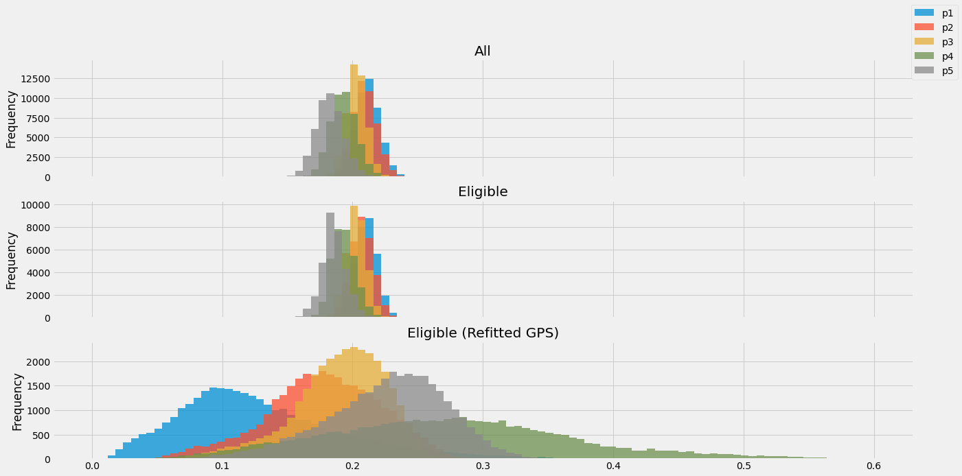 Figure 2: Propensity scores histograms for (top to bottom): all samples, eligible samples, and eligible samples after refitting their GPS scores.
Experiments
Our intention is to check whether naive methods (i.e., intended to handle binary treatment setting) are sufficient for estimating the causal effect in multiple treatment setting. For evaluating the covariate adjustment methods, we have used the two variants of our dataset (denoted in Table 2 as All, and Common support respectively). Due to computational reasons, we evaluate the matching method only on the eligible samples. To compare these methods, we choose Mean Absolute Error (MAE) as our evaluation metric. For computing the estimators we assisted with scikit-learn [4].
Results
| Dataset | All samples | Common support | |||||
|---|---|---|---|---|---|---|---|
| Setup (features used) | Covariates | Covariates + Propensity scores | Propensity scores | Covariates | Covariates + Propensity scores | Propensity scores | |
| Learner | Classifier | ||||||
| S-Learner | LogisticRegression | 0.040844 | 0.040844 | 0.040844 | 0.041382 | 0.041382 | 0.041382 |
| MLPClassifier | 0.040693 | 0.039683 | 0.039253 | 0.041458 | 0.040725 | 0.042266 | |
| RandomForestClassifier | 0.042915 | 0.042789 | 0.042688 | 0.043074 | 0.043377 | 0.043427 | |
| Linear SVM | 0.041728 | 0.041728 | 0.041728 | 0.042266 | 0.042266 | 0.042266 | |
| T-Learner | LogisticRegression | 0.021183 | 0.021183 | 0.021183 | 0.020985 | 0.020985 | 0.020985 |
| MLPClassifier | 0.019593 | 0.018576 | 0.018506 | 0.018881 | 0.017955 | 0.017843 | |
| RandomForestClassifier | 0.010837 | 0.010071 | 0.012261 | 0.010359 | 0.010289 | 0.009256 | |
| Linear SVM | 0.011573 | 0.011573 | 0.011573 | 0.012611 | 0.012611 | 0.012611 | |
| Setup (features used) | Covariates | Covariates + Propensity scores | Propensity scores | |
|---|---|---|---|---|
| Distance | Calipher | |||
| Manhattan | 0.05 | 0.046972 | ||
| 0.1 | 0.064699 | |||
| None | 0.007786 | 0.007876 | 0.092390 | |
| Euclidean | 0.05 | 0.064810 | ||
| 0.1 | 0.079215 | |||
| None | 0.005616 | 0.005878 | 0.084655 |
| Features | Covariates | Covariates + Propensity scores | |
|---|---|---|---|
| Distance | Calipher | ||
| Manhattan | 10 | 0.005496 | 0.005878 |
| Euclidean | 10 | 0.005616 | 0.005878 |
| 2.5 | 0.010433 | 0.010779 | |
| 5 | 0.005524 | 0.005788 |
Considering the Covariate Adjustment results in Table 2, we can observe how Random Forest classifier with propensity scores as features beats other methods,
when evaluated on the common-support enforced dataset. Additionally, we observe how T-Learners perform better than S-Learners.
While for the matching methods results (Table 3 and Table 4), nearest neighbor algorithms based on covariates as features get
the best results. Further, we observe that matching on covariates or, propensity scores plus covariates is better than matching based
only on propensity scores. Finally, we can also notice how optimizing the Calipher value have slightly improved our estimations with Manhattan distance,
which also yielded the most accurate result.
The results demonstrate that generally (or at least for the eligible samples dataset) matching algorithms outperform covariate adjustment. Perhaps the reason is that covariate adjustment method requires the model to be well specified, as described earlier in the methods section.
Conclusions and Future work
This technical report provides some empirical evidence that methods which were intended to handle binary treatment perform well in a multiple treatment setting. To further check our findings, we may experiment with additional types of datasets, possibly with larger treatment domains (and larger features domains accordingly). An interesting question is whether the effectiveness of these methods remain decent even when increasing the number of treatments. As follows from the results and in the spirit of [6], extending the experiments with matching algorithms may be a good future direction as well. Specifically, we can match subjects with other distances types (e.g., Mahalanobis distance), and choose different methods for enforcing common support. Furthermore, with a larger treatment domains, it would be interesting to compare our results to the specialized (multi treatment) matching algorithms introduced in [6]. Another possible future direction is to examine the training of $k$ causal forests [7] for each treatment group, and its extension to the multiple treatment setting [8].
Acknowledgment
This work was completed as a final project as part of the “Introduction to Causal Inference” course by Uri Shalit and Rom Gutman, which took place at the Technion.
A special thanks goes to my friend Guy Rotman for providing his helpful feedback on this post.
References
-
Lopez, Michael J., and Roee Gutman. “Estimation of causal effects with multiple treatments: a review and new ideas.” Statistical Science 32.3 (2017): 432-454.
-
Sekhon, Jasjeet S. “The Neyman-Rubin model of causal inference and estimation via matching methods.” The Oxford handbook of political methodology 2 (2008): 1-32.
-
Chen, H., Harinen, T., Lee, J.-Y., Yung, M., and Zhao, Z. (2020). Causalml: Python package for causal machine learning.
-
Pedregosa, F., Varoquaux, G., Gramfort, A., Michel, V., Thirion, B., Grisel, O., Blondel, M., Prettenhofer, P., Weiss, R., Dubourg, V., Vanderplas, J., Passos, A., Cournapeau, D., Brucher, M., Perrot, M., and Duchesnay, E. (2011). Scikit-learn: Machine learning in Python. Journal of Machine Learning Research, 12:2825–2830.
-
Künzel, S. R., Sekhon, J. S., Bickel, P. J., and Yu, B. (2019). Metalearners for estimating heterogeneous treatment effects using machine learning. Proceedings of the national academy of sciences, 116(10):4156–4165.
-
Scotina, A. D. and Gutman, R. (2019). Matching algorithms for causal inference with multiple treatments. Statistics in medicine, 38(17):3139– 3167.
-
Wager, S. and Athey, S. (2018). Estimation and inference of heterogeneous treatment effects using random forests. Journal of the American Statistical Association, 113(523):1228–1242.
-
Lechner, M. (2018). Modified causal forests for estimating heterogeneous causal effects. arXiv preprint arXiv:1812.09487.