Research project: CNF formula entropy approximation, applied to STS model counter as patch
In this blog post I describe a patch I have written over SearchTreeSampler [1], a model counter for SAT instances. My patch leverages its uniform solution sampling method to compute the entropy of CNF formula, a new property of SAT instances defined below.
SAT is a decision problem, meaning the algorithm that solve it should return yes or no. Without diving into definitions of complexity classes I’ll just note that SAT is very important problem, because other similar hard problems (in the sense of their hardness) could be reduced to SAT. More formally it is considered to be in NP-Complete complexity class [Cook-Levin 1971] - some computer science background is required.
There is also an annual competition for SAT solvers (programs that solve the SAT problem) which are heavily used in the industry on the domain of formal verification.
Preliminaries
SAT
Let \( X_1 ,… X_n \) be boolean variables
A boolean formula \( \varphi \) is said to be in CNF if it’s a logical conjunction of a set of clauses \( C_1,…,C_n \), where each clause \( C \) is a logical disjunction of a set of literals (a constraint over some variable, positive or negative). An example of a clause is: \( (x_1 \vee \neg x_2) \)
SAT problem is defined as deciding whether there exists an assignment that satisfies \( \varphi \)
An example: \( \varphi=(x_1 \vee \neg x_2 \vee x_3)\wedge(x_4 \vee \neg x_1)\wedge(x_2 \vee \neg x_3) \)
Satisfying assignment: \( { x_1=1,x_2=1,x_3=1,x_4=1 } \)
\( \Longrightarrow \varphi \) is SATISFIABLE
- Note that industrial formulas could easily have millions of variables and clauses.
Model counting
Model counting is actually even harder than SAT, it is believed to reside in $#P$ complexity class [M. R. Garey and D. S. Johnson 1979]. Basically in SAT we would like to decide if there exists a solution, while in model counting we want to find out how many solutions there are. Let’s define it formally:
Let \( V \) be the set of boolean variables of \( \varphi \) and let be the set of all possible assignments to these variables
An assignment \( \sigma \in \sum \) is a mapping that assigns a value in \( {0,1} \) to each variable in \( V \)
Define the weight function \( w(\sigma) \) to be 1 if \( \varphi \) is satisfied by \( \sigma \) and 0 otherwise
In this context is the actual number of solutions to \( \varphi \)
I will use the previous example to elaborate this, we already seen the assignment $\sigma = {1,1,1,1}$ is satisfying $\varphi$. All in all there could be total of $2^4$ assignments, calling a model counter for this instance returns 7 solutions.
As mentioned earlier, STS is an approximate model counter, while there are also exact counters available. Counting is hard, therefore if our interest is analyzing hard (or industrial-like) instances, we must consider using approximation methods.
- I use the terms models/solutions interchangeably
Entropy
In our research work [2] we define the entropy for CNF (Conjunctive Normal Form) formulas, which are simply normalized SAT instances. Since algorithms for solving it are mostly relied on heuristics (SAT is NP-Hard), our motivation was to find a measure that quantifies the hardness of a single instance, that hopefully could explain why some heuristics are better than others. Hence we turned to experimenting with Shannon’s entropy [3], let’s define it formally in our context:
Let be a propositional CNF formula, its set of variables and its set of literals.
If is SATISFIABLE, we denote by , for , the ratio of solutions to that satisfy . Hence for all , it holds that
The entropy of a variable is defined by:
Definition: The entropy of a satisfiable formula is the average entropy of its variables.
 Figure 1: Entropy reflects the freedom we have in assigning the variables
Reminder: Model counting is a problem, entropy is hard to compute and requires calls to model counter (as number of variables in input formula).
STS and patch explained
Hashing and optimization
STS - Search Tree Sampler [1], is an approximate model counter. It uses hashing and optimization technique in order to count solutions. In the context of model counting:
- Hashing means that on each ‘level’ the algorithm explores, we shrink the solutions space.
- Optimization means using a SAT solver as an oracle to tell the algorithm if solutions still exist after shrinking.
See figure below, which describes how the counter repeats this method until no solutions exists, which in turn allows us to approximate number of solutions. This technique is also common in probabilistic inference problems.
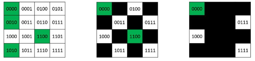 Figure 2: Approximate model counter: on each step $m$ (starting from $m=0$) randomly partition half of $\Sigma$, then invoke a SAT solver to decide if solutions still exist, if not the algorithm halts. Number of models is then approximated using the number of total iterations $m$. In the case illustrated, after 2 iterations solutions still exist and the next iteration would lead to halt, hence the checked formula has $2^2$ solutions (green cells depicted on left). Notice there could be a case where the counter may randomly partition a solution cell, and then the algorithm will stop ahead of time, resulting with a non-correct $m$. Figure taken from [5]
Computing entropy requires to compute for each literal, is the ratio of solutions that the literal appears in, out of all formula’s solutions. So technically if we have a decent amount of uniform solutions, we can approximate the variables entropy. STS works by sampling uniform (controlled by a parameter) solutions. I took advantage of this mechanism and on each run of the algorithm I recorded those uniform solutions, in order to cheaply approximate the entropy, with only one run of STS instead of runs (input size of the formula).
Patch explained
STS is built on top of Minisat [4], the algorithm is implemented on Main.cc. In the following I describe my patch, you can open the code and follow:
First I added the needed variables
// a vector for counting #(x) and #(!x)
std::vector<int> varSolCountPos; // counter for pos
std::vector<int> varSolCountNeg; // counter for neg
std::vector<double> rvPos;     // vector for r(v)
std::vector<double> rvNeg;
std::vector<double> ev;      // vector for e(v)
Then initialized them:
varSolCountNeg.resize(var_num);
varSolCountPos.resize(var_num);
rvPos.resize(var_num);
rvNeg.resize(var_num);
ev.resize(var_num);
for (int iter=0; iter<var_num; iter++)
{
  varSolCountPos[iter] = 0;
  varSolCountNeg[iter] = 0;
  rvPos[iter] = 0;
  rvNeg[iter] = 0;
  ev[iter] = 0;
}
Inside the loop for outputting solutions we count the number of times each literal appear in the solutions:
// compute #(x) and #(!x)
if (OutputSamples[l][i] == 1)
{
	varSolCountPos[i] += 1;
} else {
	varSolCountNeg[i] += 1;
}
When we have the counts we can use them to approximate and the entropy of each variable, notice I also keep a file to write output:
// file for outputting entropies
FILE * pFile;
// produce filename
char* filename;
char* buff;
buff = basename(argv[1]);
filename = strcat(buff, ".entropy.out");
pFile = fopen(filename, "w");
// header
fprintf(pFile, "Var,TotalSols,PosLitSols,NegLitSols,EntropyShan\n");
// compute r(v) and e(v)
for (int iter=0; iter < var_num; iter++)
{
  int total = varSolCountPos[iter] + varSolCountNeg[iter];
  double logrv = 0;
  double logrvBar = 0;
  rvPos[iter] = (double)varSolCountPos[iter] / total;
  rvNeg[iter] = 1-rvPos[iter];
  if (rvPos[iter] != 0 && rvNeg[iter] !=0)
  {
    logrv = log2(rvPos[iter]);
    logrvBar = log2(rvNeg[iter]);
  }
  else
  {
    if (rvPos[iter] == 0)
      logrv = 0;
    if (rvNeg[iter] == 0)
      logrvBar = 0;
  }
  ev[iter] = -( (rvPos[iter]) * (logrv) ) - ( (rvNeg[iter])*(logrvBar) );
  int varnum = iter+1;
  fprintf(pFile, "%d,%d,%lf,%lf,%lf\n", varnum, total, rvPos[iter], rvNeg[iter], ev[iter]);
}
Computing the formula entropy is done by averaging the variables entropy:
// compute entropy

double sumEntropy = 0;
for (int iter=0; iter < var_num; iter++)
{
  sumEntropy += ev[iter];
}

double lastEntropy = sumEntropy / var_num;
Finally printing the averaged entropy, and handling the output file:
printf("Estimated entropy: %lf\n", lastEntropy);
fprintf(pFile, "#Estimated entropy: %lf\n", lastEntropy);
fclose(pFile);
printf("Output file: %s\n", filename);
Sanity check
Let’s examine a simple formula with 3 variables:
$ \varphi = (X_1 \vee X_2 \vee X_3) \wedge (X_1 \vee \neg X_2 \vee X_3) \wedge (X_1 \vee X_2 \vee \neg X_3)$
This is how its CNF looks like:
p cnf 3 3
1  2  3  0
1  -2  3  0
1  2  -3  0
We can write it down and see that there are total 5 solutions:
{ (1,0,0), (1,0,1), (1,1,0), (1,1,1), (0,1,1) }
Ratios of each literal (number of times it appears in solutions): {r(1) = 4/5, r(-1) = 1/5, r(2) = 3/5, r(-2) = 2/5, r(3) = 3/5, r(-3) = 2/5}
In this scenario of tiny formula the approximator sampled 50 solutions. Some of the solutions are identical of course, but usually it isn’t the case where we handle larger formulas. In particular the samples should be sampled uniformly (randomly). Let’s take a look of output:
Var,TotalSols,PosLitSols,NegLitSols,EntropyShan
1,50,0.800000,0.200000,0.721928
2,50,0.600000,0.400000,0.970951
3,50,0.600000,0.400000,0.970951
#Estimated entropy: 0.887943
The ratios (PosLitSols/NegLitSols) converged exactly to the correct values.
References
-
Stefano Ermon, Carla Gomes, and Bart Selman. Uniform Solution Sampling Using a Constraint Solver As an Oracle. UAI-12. In Proc. 28th Conference on Uncertainty in Artificial Intelligence, August 2012.
-
Dor Cohen, Ofer Strichman, The Impact of Entropy and Solution Density on Selected SAT Heuristics. Entropy 2018, 20, 713.
-
Shannon, C.E. (1948), “A Mathematical Theory of Communication”, Bell System Technical Journal, 27, pp. 379–423 & 623–656, July & October, 1948.
-
Niklas Een, Niklas Sörensson , MiniSat - A SAT solver with conflict-clause minimization, SAT Poster 2005
-
Perturbations, Optimization, and Statistics (chapter 9) - edited by Tamir Hazan, George Papandreou and Daniel Tarlow, MIT press 2016
- Seminar talk I have presented, which summarizes the relevant chapter on [5].